The demand for transparency in sustainable development from investors and customers has grown over the years.

Investors have placed an increased emphasis on the sustainability of the business when assessing the value and resiliency of an organization.

Therefore, more and more organizations invest resources to build capabilities for sustainability reporting and determine the best strategies for a sustainable supply chain.

In this article, we will introduce a simple methodology to report the CO2 emissions of your Distribution Network using Python and PowerBI.

I. CO2 emissions formula for transportation

Definition

Based on the GHG Protocol corporate standard (Link), greenhouse gas emissions are classified into three scopes:

• Scope 1: direct emissions released to the atmosphere because of company’s activities (Company’s facilities like manufacturing plant/warehouses, company’s vehicles)
• Scope 2: indirect emissions from the generation of purchased energy
  (purchased electricity, gas, ..)
• Scope 3: all indirect emissions (out of scope 2) occurring in the value chain of the company (Transportation, Waste of Operations, Business Travels, …)

In this article, we will focus our attention on the Scope 3 calculations related to downstream transportation.

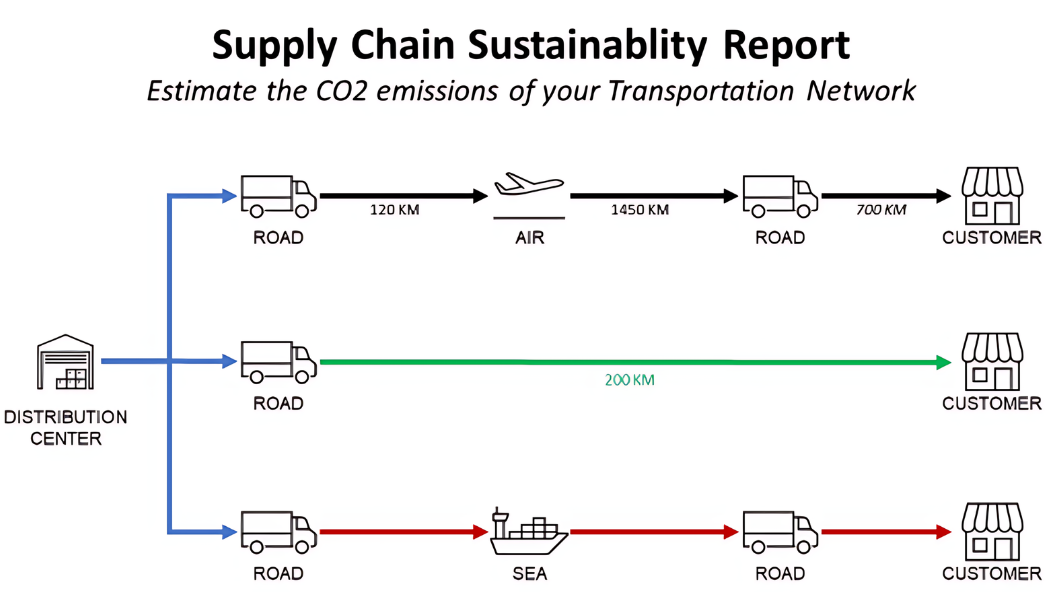
What is the environmental impact of your distribution network?

Formula

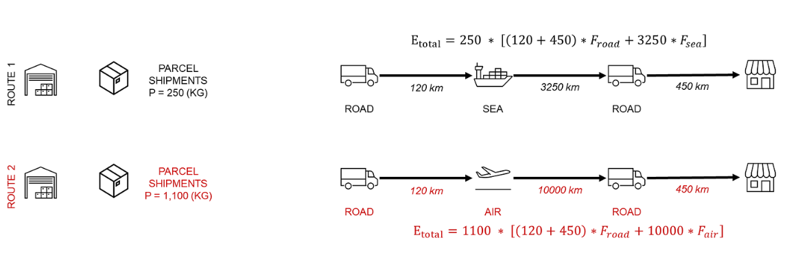
Following the protocol of the French Environmental Agency Ademe (Link), the formula to estimate the CO2 emissions of transportation is:

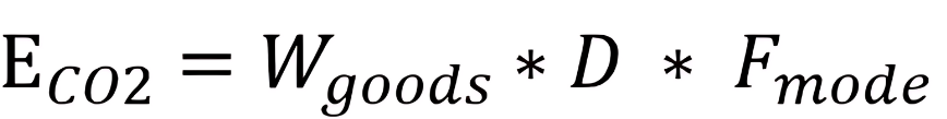
With,

This formula provides a gross estimation of the CO2 emissions without requiring a high level of granularity of transportation data.

A more accurate approach would be to estimate the CO2 emissions of each delivery considering the model of the vehicle (truck, container carrier, plane or train) and the filling rate.

II. Data processing with Python

Based on this formula, we can now start to collect data to calculate the emissions.

Import shipped order lines

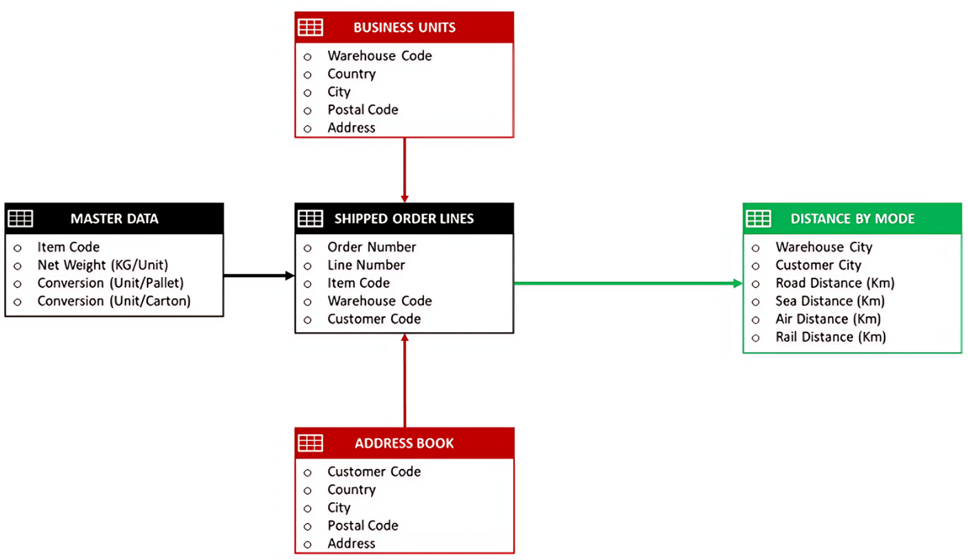
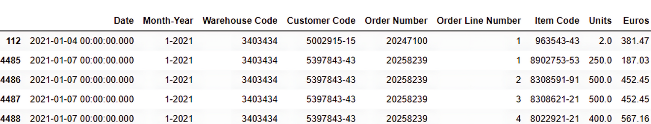
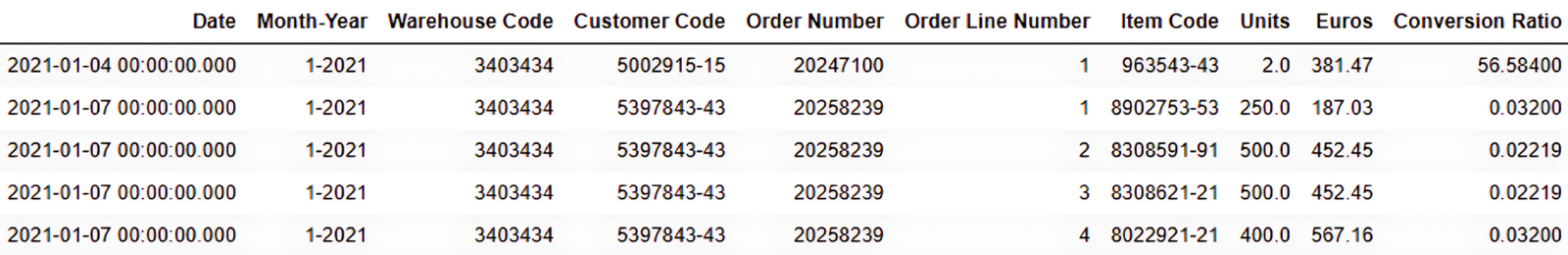
Let‘s start by extracting from our ERP (or WMS) the shipped order lines: all purchased orders of your customers that have been shipped from your warehouses.

This dataset includes

• Order information: Order Number, Line Number
• Item Code: Identification number of the item in the master data
• Warehouse Code: the business unit from where these orders are shipped (Distribution Center, Factory)
• Customer Code: the final destination where the orders are delivered (Store, Distribution Center)

Code

import numpy as np
import pandas as pd
import matplotlib.pyplot as plt
import datapane as dp

# Volumes per day
df_day = pd.read_csv('data/volumes per day.csv')
# Bar Plot: Orders/Lines
orderlines = ([dp.Plot(df_day[df_day['WEEK'] ==wk].plot.bar(figsize=(8, 6), 
edgecolor='black', x='DAY', y=['ORDERS', 'LINES'], color=['tab:blue', 'tab:red'], legend= True), 
label = wk)
for wk in df_day['WEEK'].unique()])
plt.xlabel('DAY', fontsize = 12)
plt.title('Workload per day (Lines/day)', fontsize = 12)
plt.show()

# Section to deploy
# Plot Orders Lines per day
dp.Report(
  dp.Page(
    dp.Select(blocks = orderlines)
  )
).upload(name='orders/lines per day')

Result

Add unit of measure conversions

The next step is to convert the quantities ordered into weight (kg).

Net Weight vs. Total Weight
Before going into the details of the calculation, we need to explain the difference between gross and net weight.

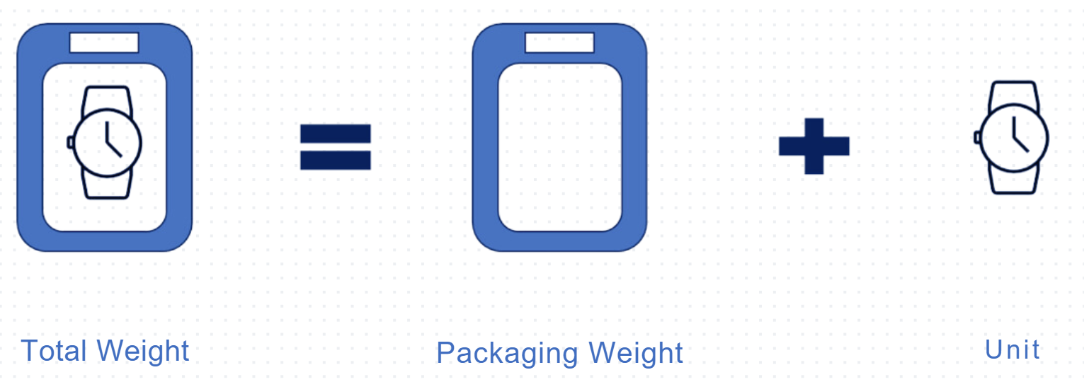
Packaging is the container used to cover your finished product. In some ERP’s master data, you may find the net weight (without packaging) and the gross weight (with packaging).

For this report, we need to make sure to take the gross weight to estimate the total weight including packaging.

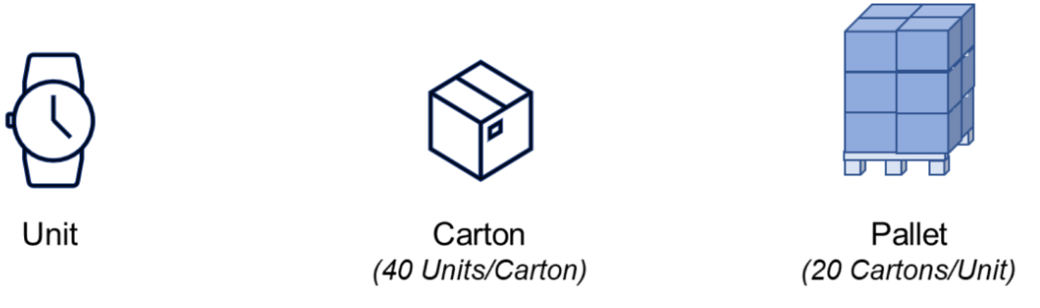
Handling Unit (Cartons, Pallet)
Depending on the order quantity, your customer can order by unit, cartons (grouping several units) or pallets (grouping several cartons).

If you are lucky enough to have the weights of cartons or pallets, you can use them if your customer is ordering full cases or full pallets.

Assumption of Mixed Cartons
For certain logistic operations, where you need to perform piece picking (Luxury, Cosmetics, E-Commerce), the quantity per order line is so low that you rarely ship full cartons.

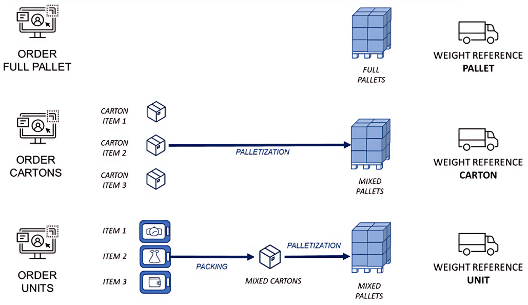
In this case, there is no point in using full cartons weight; we can only rely on the total weight per unit. For our example, we will assume that we are in this situation.

Code

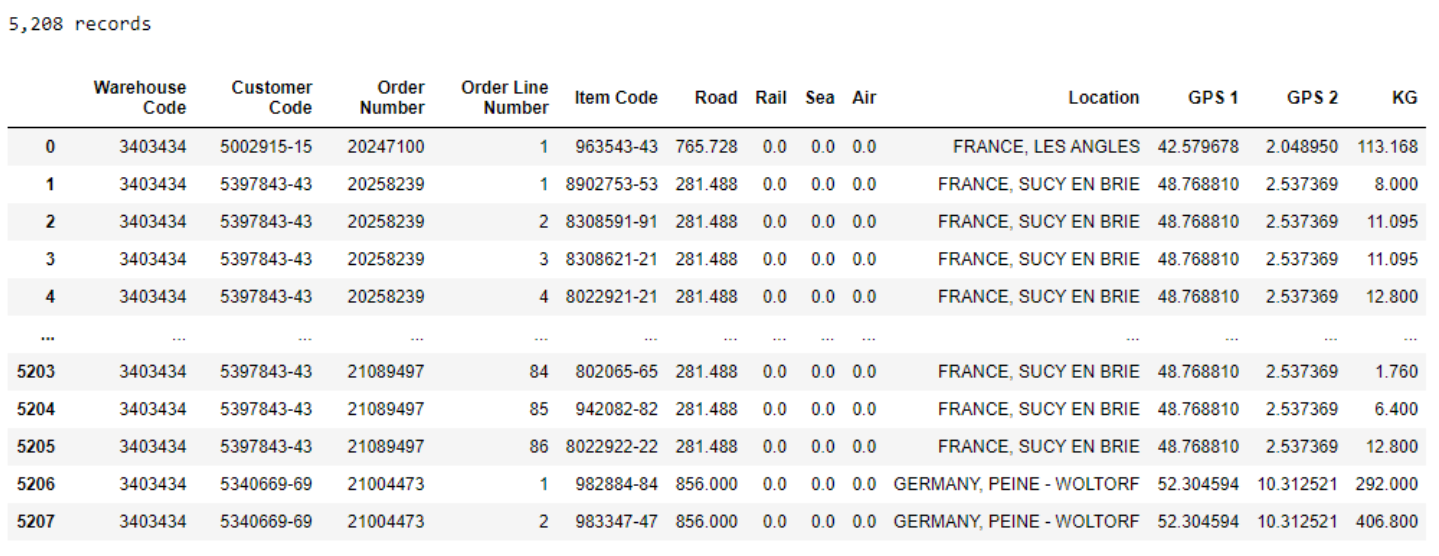
df_uom = pd.read_csv('Data/uom_conversions.csv', index_col = 0)
print("{:,} Unit of Measure Conversions".format(len(df_uom)))

# Join
df_join = df_lines.copy()
COLS_JOIN = ['Item Code']
df_join = pd.merge(df_join, df_uom, on=COLS_JOIN, how='left', suffixes=('', '_y'))
df_join.drop(df_join.filter(regex='_y$').columns.tolist(),axis=1, inplace=True)
print("{:,} records".format(len(df_join)))
df_join.head()

Results

Distances Collections and GPS Locations

We need to collect the distance by mode:

• Air Freight
• Sea Freight
• Road Transportation: Trucks
• Rail Transportation: Trains

We will also add the GPS locations of the destination for our PowerBI reporting.

Code

df_dist = pd.read_csv('Data/' + 'distances.csv', index_col = 0)
# Location
df_dist['Location'] = df_dist['Customer Country'].astype(str) + ', ' + 
df_dist['Customer City'].astype(str)
# Add GPS
df_gps = pd.read_csv('Data/' + 'gps_locations.csv', index_col = 0)
print("{:,} Locations".format(len(df_gps)))
# Merge GPS + Location
df_dist = pd.merge(df_dist, df_gps, on='Location', how='left', 
suffixes=('', '_y'))
df_dist.drop(df_dist.filter(regex='_y$').columns.tolist(),
axis=1, inplace=True)
# Merge with join records
COLS_JOIN = ['Warehouse Code', 'Customer Code']
df_join = pd.merge(df_join, df_dist, on = COLS_JOIN, how='left', 
suffixes=('', '_y'))
df_join.drop(df_join.filter(regex='_y$').columns.tolist(),axis=1, 
inplace=True)
print("{:,} records".format(len(df_join)))

III. CO2 calculation

1. Final calculation of the CO2 emissions

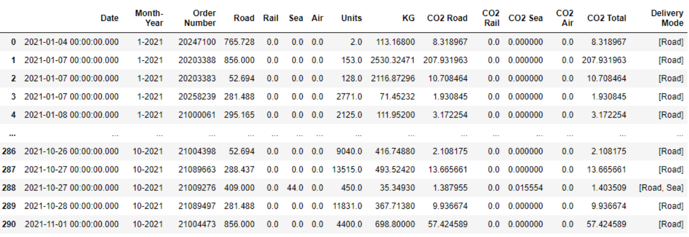
We have now all the information needed to be gathered in a single DataFrame. We can start to calculate the CO2 emissions using emissions factors associated with your transportation network.

Sum the weight by Order
For reporting purposes, let us calculate the CO2 emissions for each order number (linked with a customer and a date).

# Calculate Weight (KG)
df_join['KG'] = df_join['Units'] * df_join['Conversion Ratio']
# Agg by order
GPBY_ORDER = ['Date', 'Month-Year', 
        'Warehouse Code', 'Warehouse Name', 'Warehouse Country', 'Warehouse City',
        'Customer Code', 'Customer Country', 'Customer City',
'Location', 'GPS 1', 'GPS 2', 
        'Road', 'Rail', 'Sea', 'Air',
        'Order Number']
df_agg = pd.DataFrame(df_join.groupby(GPBY_ORDER)
[['Units', 'KG']].sum())
df_agg.reset_index(inplace = True)
# CO2 Emissions Calculation
dict_co2e = dict(zip(['Air' ,'Sea', 'Road', 'Rail'], [2.1, 0.01, 0.096, 0.028]))
MODES = ['Road', 'Rail','Sea', 'Air']
for mode in MODES:
    df_agg['CO2 ' + mode] = df_agg['KG'].astype(float)/1000 * 
df_agg[mode].astype(float) * dict_co2e[mode]
df_agg['CO2 Total'] = df_agg[['CO2 ' + mode for mode in MODES]].sum(axis = 1)
# Mapping the delivery Mode
df_agg['Delivery Mode'] = df_agg[MODES].astype(float).apply(
    lambda t: [mode if t[mode]>0 else '-' for mode in MODES], axis = 1)
dict_map = dict(zip(df_agg['Delivery Mode'].astype(str).unique(), 
  [i.replace(", '-'",'').replace("'-'",'').
replace("'",'') for i in df_agg['Delivery Mode'].astype(str).unique()]))
df_agg['Delivery Mode'] = df_agg['Delivery Mode'].astype(str).map(dict_map)

Final results

2. What if you don’t have 100% of the distances?

A major challenge here is to get the distances if you have several thousand delivery locations.

If you are not able to collect 100% of the distance from your carriers, you can:

• Get the road distances using Google Maps API
• Estimate the distance using the Haversine formula
• Compute the average distance of your top customers (in Euros) and apply the average to the locations without distances

3. What if you don’t have 100% of the weight conversions?

In some cases, the master data is not updated and you cannot get the unit of measure conversions for all the items.

In that case, you can

1. Focus your data collection efforts on the high runners (turnover)
2. Estimate the weight per euro for these items (kg/euros)
3. Apply the average ratio on the c remaining items without conversions to get their weight

VI. Example of visualization using PowerBI

Bubble map with size = f(CO2 Total)

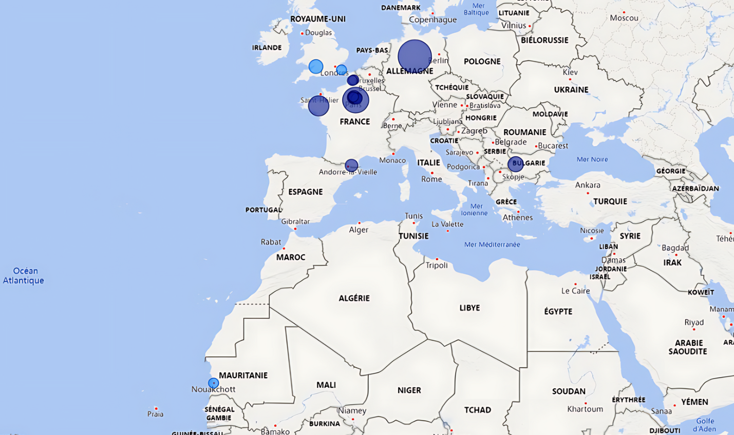
Visual Insights
You can observe where you have the majority of CO2 emissions (large bubbles) with a colour coding by transportation mode.

Split by Country Destination and Item Code

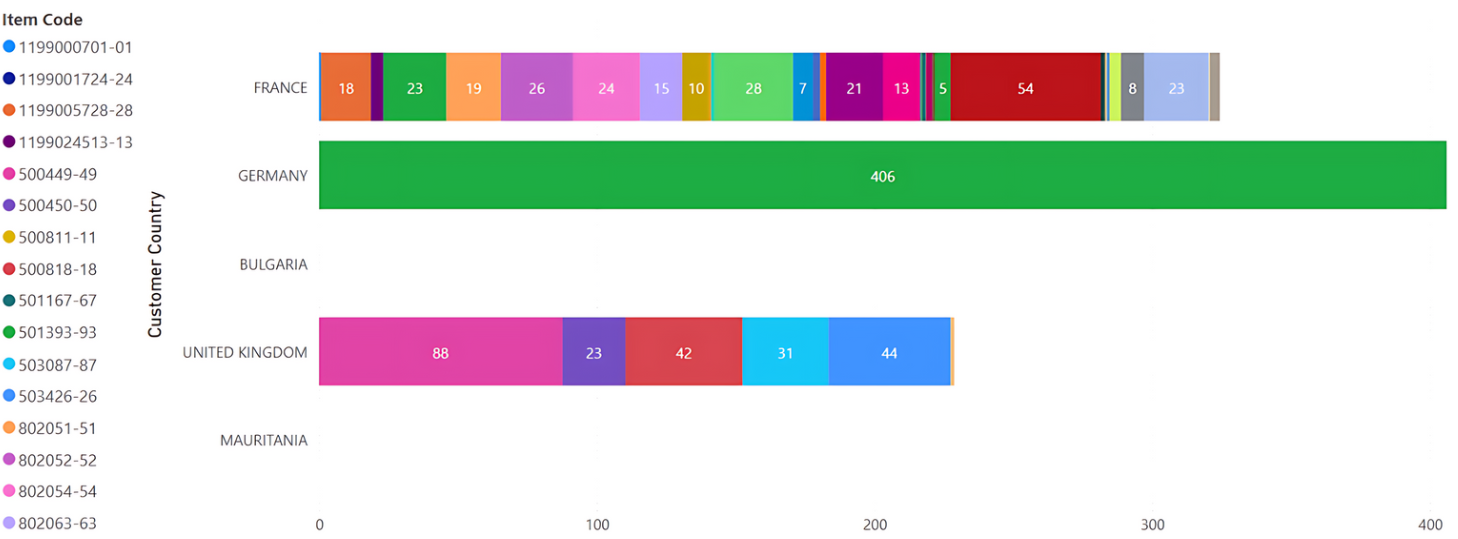
Product Portfolio Insights
For each market, which item has the highest environmental impact?

CO2 = f(Turnover) by City Destination

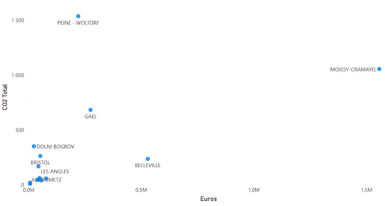
Financial Insights
The impacts of your future efforts for CO2 Emissions reductions on the profitability will probably be higher for the customers in PEINE-WOLTORF.

Next Steps

After measuring your emissions, a potential next step could be to optimize your Distribution Network using a methodology presented in the next article.

References

[1] GHG Protocol corporate standard, Greenhouse Gas Protocol, Link

[2] French Environmental Agency Ademe, Bilan GES, Link

[3] Github Repository with source code and data, Samir Saci, Link