
· 6 min read
Real-world reinforcement learning applications are hard to find. This article gives a high-level overview of building an RL agent aimed to optimize the energy use. The article is divided into following sections:
- Problem setting — defining the problem and the goal.
- Building a simulation environment — description of how the training environment was built including the representation of the observation space, action space and rewards of the agent.
- Training process — frameworks, algorithms used in the training and the chart of the training process.
- Agent in action — an example of how the trained agent makes decisions.
- Conclusion — final thoughts.
Problem setting
We have an household that generates its own solar energy with 12 kWp unit and is able to store this energy in a home battery (Tesla Powerwall 2 with 13 kWh capacity) which can be controlled through API. The electricity contract of the household is based on day-ahead market prices and the storage device can also be used to participate in aFRR-up/secondary reserve market.
Our goal is to train an agent that minimizes the energy cost of a household by controlling the battery considering the energy markets (day-ahead market, frequency markets), the local conditions (e.g. the baseload of the household) and user preferences (e.g. battery level can’t go below certain threshold).
Building a simulation environment
In reinforcement learning, the agent learns by making actions in an environment, receiving rewards/penalties for those actions and modifying its action pattern (policy) accordingly.
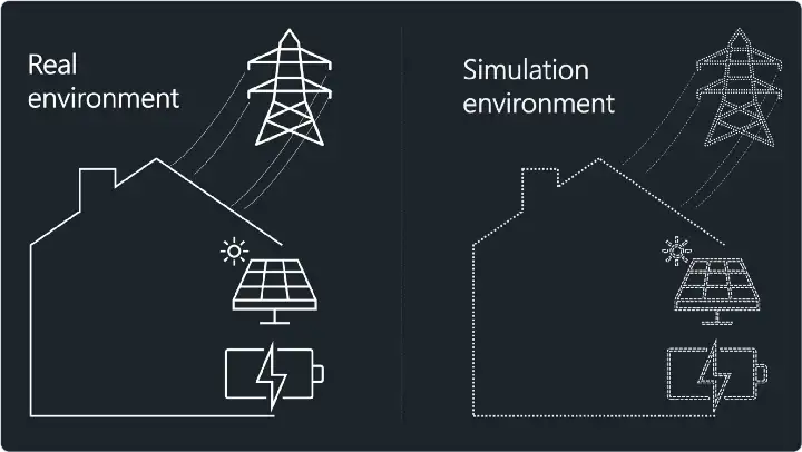
One could either use the real environment (the real household and the energy markets) or simulated environment. In this project, a simulation environment was built, using the OpenAI Gym as a framework.
Developing the simulation environment for the energy decision agent involved the following steps:
- Representing the current situation (the state) of the environment numerically. The state representation needs to involve all of the information that our agent needs for training.
- Representing the possible actions (things that our agent can make with our battery) numerically. Representing and updating the current state of the home battery.
- Developing a logic of what it means to make a specific action in the environment. In other words, expressing what would happen with the household, battery and the energy cost when specific action is carried out by the agent.
In total, the programmatical representation of our environment included ca 700 lines of code (including the helper functions). Next, I’ll explain some of the key parts of the environment.
Representing the current state/observation
The state/observation is a numerical representation of the current situation. In our project, this means representing the current state of energy markets, household and the assets.
Initial representation of the current state
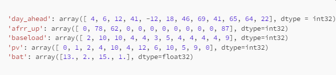
Our initial (unmodified) observation space consists of the following information:
- 12-hour forecast of day-ahead energy market prices,
- 12-hour forecast of afrr_up frequency market prices,
- 12-hour forecast of household’s consumption,
- 12-hour forecast of local solar production,
- The information about the battery (vector of length 4): the capacity of the battery (e.g. 13 kWh); the current charge level of the battery (e.g. 2 kWh); the maximum charge power (e.g. 5 kW); the minimum allowed charge level (e.g. 1 kWh).
The code block below represents an example of the unmodified observation components: we have 12 forecasted values of day-ahead and afrr-up market prices, the same number of corresponding baseload and pv-product values and 4 values that represent the information about the battery.
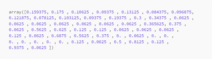
Modified observation space
The initial observation representation was modified in order to make it easier to handle by the neural network that our agent uses for learning. Each observation was normalized (represented between 0 and 1) and flattened (given as a single vector instead of five different vectors). The modified observation looks like this:
Action space
Action space represents the decisions (actions) that the agent can make. Our energy decision agent has discrete action space of length 6.
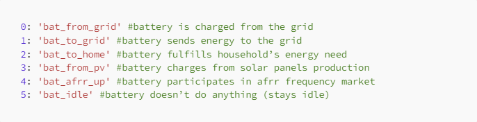
Each value (from 0–5) corresponds to one of the actions that the agent can do with the battery. Each action affects the State-of-Charge of the battery and has a corresponding cost/benefit.
Complexity: One episode is 24 hours and we have 6 actions to select for each hour. We have 4 738 381 338 321 616 896 (4.7 quintillion) possible ways to use this battery in a single episode.
Reward
The agent is rewarded on each step and the reward equals the energy cost that the household experiences. For example, if the agent decides on action value 0: ‘bat_from_grid’, then the maximum possible amount of energy is charged from the grid to the battery and the agent receives the reward that equals to: charging cost + household baseload cost + revenue from pv production + …
The goal of the agent was to maximize the reward for the 24 hours timespan (that is: 24 hours was defined as a single episode).
Training process
During the training phase, the agent makes actions in the simulated environment and tries to find the action plan that is monetarily most beneficial to the household. In this project, the agent was represented by the RLLIB’s implementation of the IMPALA algorithm. IMPALA enables to train the agent of multiple CPU cores simultaneously. The setup in this project included 4 cores/workers and 3 environments per worker.
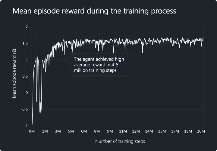
The image below represents the mean episode reward (calculated as a mean of 100 episodes) during the training process. We can see that the agent evolved very quickly but the stability of the policy (its decision pattern) was rather low during the first two million steps of training. At the last stages of the training, our agent was able to consistently retrieve the mean reward of 1.5–1.6 € per episode.
Agent in action
As a final step, let’s take a look at the actions that our agent proposes for a sample 24-hour period (the image below). The Day-ahead and Afrr-up columns represent the market prices on those hours. The baseload and the PV represent the regular consumption and the PV-production of the household (in kWh). The Action column indicates the action/decision that is proposed by our energy decision agent and the SoC column shows the battery level (in kWh) at the end of the hour (after carrying out the proposed action).
The first highlighted region of the table shows how our agent is able to allocate the battery on the afrr-up market during the high-priced hours (hours 21, 22, 0) and charge from the grid during the hours when the day-ahead prices are low (hours 28 and 4).
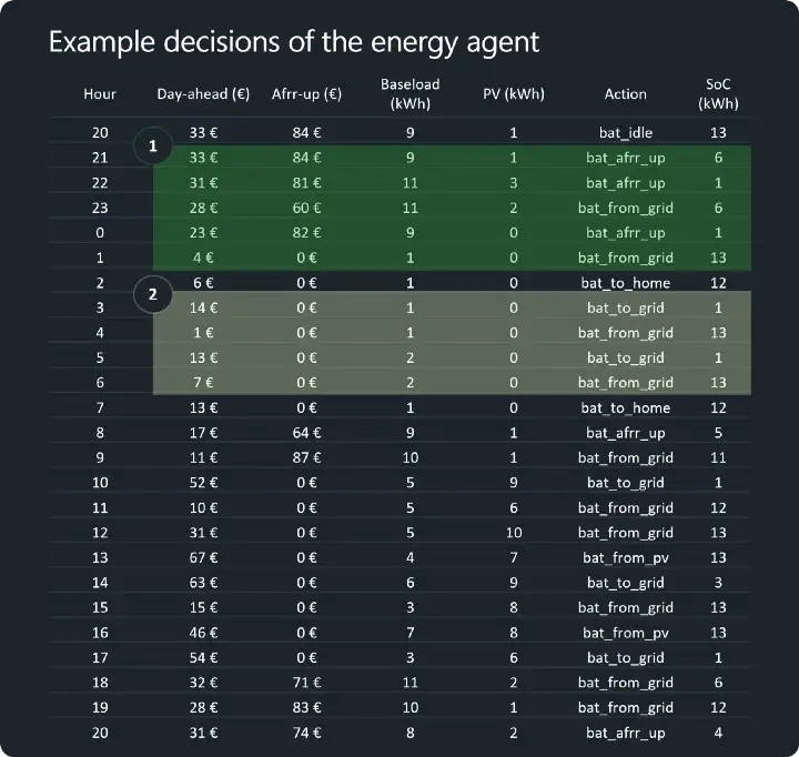
The second highlighted region indicates the pure market price arbitrage by our agent — discharging with the high-priced hours (hours 3 and 5) and charging during the low-priced hours (hours 4 and 6).
Conclusion
As a conclusion, I would like to highlight the following aspects:
- The reinforcement learning can be used to train an energy decision agents.
- The key of building a real-world application of reinforcement learning is in building a training environment that closely resembles the physical world.
- RL agents doesn’t guarantee optimality and can be very sensitive to the small changes in the environment.
- Think! Maybe your problem could be solved with a simpler method!
This article is also published on Medium. Future Thought Leaders is a democratic space presenting the thoughts and opinions of rising Sustainability & Energy writers, their opinions do not necessarily represent those of illuminem.


